More on Tableaux
Although we represented tableaux as trees in the previous post, the way we interacted with these trees makes clear that the really crucial part of a tableau-tree is that it is a way to represent a set of branches. In building these tableaux, we operated exclusively on branches - we chose a particular branch, and expanded it. Expanding a branch amounts to replacing it with new branches (sometimes just one, sometimes two). The (unfinished) tableau below has three branches.
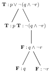
Figure 1: A tableau qua tree with three branches
The three branches of the above tree are as follows:
| Branch | Content |
|---|---|
| branch 1 | \(\{\textbf{T}:p \vee \neg (q \wedge \neg r),\textbf{T}: p\}\) |
| branch 2 | \(\{\textbf{T}:p \vee \neg (q \wedge \neg r),\textbf{T}:\neg (q \wedge \neg r), \textbf{F}: q \wedge \neg r, \textbf{F}:q\}\) |
| branch 3 | \(\{\textbf{T}:p \vee \neg (q \wedge \neg r),\textbf{T}:\neg (q \wedge \neg r), \textbf{F}: q \wedge \neg r, \textbf{F}:\neg r\}\) |
Each of these branches represents a potential situation which makes the formula at the root have the appropriate truth value. The first branch represents a situation in which the atom \(p\) is true, and the complex formula \(p \vee \neg (q \wedge \neg r)\) is as well. This first branch (in the tree, this is the leftmost branch) has no productive formulae, and so we are done with it. The second branch (the one in the middle of the tree) also has no productive formulae, and it is done as well. The third branch (rightmost in the tree) has a single productive formula, \(\textbf{F}:\neg r\). There is no way to tell which formulae are productive or not given a branch in isolation. Since we no longer use non-productive formula, it is easiest to just remove formulae once they have been expanded. With this agreement, we would write our three branches above (indicating only the formulae which have not yet been expanded) as follows:
| Branch | Content |
|---|---|
| branch 1 | \(\{\textbf{T}: p\}\) |
| branch 2 | \(\{\textbf{F}:q\}\) |
| branch 3 | \(\{\textbf{F}:\neg r\}\) |
Eliminating the unproductive non-atomic formulae helps us understand the situations described by the branches better. Branch 1 corresponds to any situation making \(p\) true. Branch 2 to any situation making \(q\) false, and branch 3 to any situation making \(\neg r\) false. Observe that, first, the branches represent sets of situations, rather than single situations. And second, the sets of situations represented by different branches needn’t be disjoint. As an example, a situation making \(p\) true and \(q\) false is described both by branch 1 and by branch 2.
As a point of comparison of our two notations for tableaux, we walk through the tableau attempting to refute the sentence \(\neg(p_{1} \wedge \neg (p_1 \wedge \neg p_{2})) \vee p_{2}\) in these two notations.
| Step | Tree | Branch set |
|---|---|---|
| 1 | 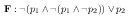 |
\(\{\textbf{F}:\neg(p_{1} \wedge \neg (p_1 \wedge \neg p_{2})) \vee p_{2}\}\) |
| 2 |  |
\(\{\textbf{F}:\neg(p_{1} \wedge \neg (p_1 \wedge \neg p_{2})), \textbf{F}:p_{2}\}\) |
| 3 | 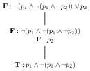 |
\(\{\textbf{T}:p_{1} \wedge \neg (p_1 \wedge \neg p_{2}),\textbf{F}:p_{2}\}\) |
| 4 |  |
\(\{\textbf{T}:p_{1},\textbf{T}: \neg (p_1 \wedge \neg p_{2}),\textbf{F}:p_{2}\}\) |
| 5 |  |
\(\{\textbf{T}:p_{1},\textbf{F}: p_1 \wedge \neg p_{2},\textbf{F}:p_{2}\}\) |
| 6 | 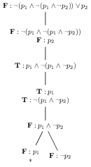 |
\(\{\textbf{T}:p_{1},\textbf{F}: p_1,\textbf{F}:p_{2}\}, \{\textbf{T}:p_{1},\textbf{F}: \neg p_{2},\textbf{F}:p_{2}\}\) |
| 7 | 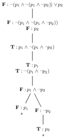 |
\(\{\textbf{T}:p_{1},\textbf{F}: p_1,\textbf{F}:p_{2}\}, \{\textbf{T}:p_{1},\textbf{T}: p_{2},\textbf{F}:p_{2}\}\) |
In step 6 we introduce our first branching node in the tree. Here we can see a major difference between the tree and the branch set representations: the branch set representation requires us to duplicate all formulae previously on the branch in both new branches. The tree representation shares these common formulae. Of course the representational advantage of the branch set representation is that keeping track of which formulae on each branch are productive is much simpler - the non-productive ones are simply removed (except atomic ones).
TL/DR
-
Please practice using this alternative representation for tableau method!
- Create a tableau qua set of branches starting with the following signed formulae:
-
\(\textbf{T}: p \vee \neg p\)
-
\(\textbf{F}: p \vee \neg p\)
-
\(\textbf{T}: (p \vee \neg q) \wedge (q \vee \neg r) \wedge (\neg p \vee r) \)
remember that conjunction is associative: you get the same truth value no matter how you parenthesize the following expression. \[p \wedge q \wedge r\ \approx\ p \wedge (q \wedge r) \equiv (p \wedge q) \wedge r\]
-
\(\textbf{F}: (p \vee \neg q) \wedge (q \vee \neg r) \wedge (\neg p \vee r) \)
-
- I claim that the following formulae are valid. Verify my claims using the tableau method!
- \(\neg (p \wedge \neg p)\)
- \(\neg (\neg p \vee q) \vee \neg (p \wedge \neg q)\)
- \(\neg ((\neg p \vee q) \wedge (p \wedge \neg q))\)
- Create a tableau qua set of branches starting with the following signed formulae:
-
Think about how implication fits into the \(\alpha\)/\(\beta\) scheme given in this post.
-
Take a gander at the code for propositional tableaux, and try to use it to verify your answers to the practice questions above!
Revisiting the tableau rules
There are two directions along which I would like to revisit our tableau rules from last time. One of them offers a conceptual unification, and the other is a perspective shift that is useful in implementing the tableau method. The tableau rules given in the previous post are repeated below for convenience, but are rephrased to talk about branches instead of trees.
- \(\textbf{T}: \neg\phi\)
- add signed formula \(\textbf{F}: \phi\) to the current branch
- \(\textbf{F}: \neg\phi\)
- add signed formula \(\textbf{T}: \phi\) to the current branch
- \(\textbf{T}: \phi \wedge \psi\)
- add signed formulae \(\textbf{T}: \phi\) and \(\textbf{T}:\psi\) to the current branch
- \(\textbf{F}: \phi \wedge \psi\)
- split the current branch into two branches, add signed formula \(\textbf{F}:\phi\) to one, and signed formula \(\textbf{F}:\psi\) to the other
- \(\textbf{T}: \phi \vee \psi\)
- split the current branch into two branches, add signed formula \(\textbf{T}:\phi\) to one, and signed formula \(\textbf{T}:\psi\) to the other
- \(\textbf{F}: \phi \vee \psi\)
- add signed formulae \(\textbf{F}: \phi\) and \(\textbf{F}:\psi\) to the current branch
Alpha and Beta rules
Despite having two rules for each formula type (one for sign T, and one for F), these six rules do either one of two things. They either extend the current branch, or split the current branch. We classify each signed formula type into one of two categories, \(\alpha\) and \(\beta\):
| \(\alpha\) | \(\alpha_{1}\) | \(\alpha_{2}\) |
|---|---|---|
| \(\textbf{T}: \phi \wedge \psi\) | \(\textbf{T}:\phi\) | \(\textbf{T}:\psi\) |
| \(\textbf{F}: \phi \vee \psi\) | \(\textbf{F}:\phi\) | \(\textbf{F}:\psi\) |
| \(\textbf{T}: \neg \phi\) | \(\textbf{F}:\phi\) | \(\textbf{F}:\phi\) |
| \(\textbf{F}: \neg \phi\) | \(\textbf{T}:\phi\) | \(\textbf{T}:\phi\) |
| \(\beta\) | \(\beta_{1}\) | \(\beta_{2}\) |
|---|---|---|
| \(\textbf{F}: \phi \wedge \psi\) | \(\textbf{F}:\phi\) | \(\textbf{F}:\psi\) |
| \(\textbf{T}: \phi \vee \psi\) | \(\textbf{T}:\phi\) | \(\textbf{T}:\psi\) |
Now we can give our tableau rules in terms of the category of signed formula as follows:
- \(\alpha\)
- add \(\alpha_{1}\) and \(\alpha_{2}\) to the current branch
- \(\beta\)
- split the current branch into two branches, add \(\beta_{1}\) to one, and \(\beta_{2}\) to the other
Revisiting the role of formulae
Let us rethink what the impact of a particular formula is on a tableau. The rules we have given tell us how to extend a branch given a signed formula. So if we have a signed formula, we are waiting for a branch from which we can construct one or more branches. Thus we can view a signed formula as a function from branches to sets of branches. As a tableau is itself just a set of branches, a signed formula is a function from branches to tableaux. A formula without a sign is then waiting for a sign and a branch to create a tableau. As a sign is just a truth value, a formula is a function from a boolean and a branch to a tableau. In other (haskellian) words:1
newtype Formula a = Formula {unFormula :: Bool -> Branch a -> Tableau a}
We can ask how each kind of formula modifies a branch, when we interpret it in this way. An atomic formula will add itself to a branch if possible, but if this results in the branch becoming invalid, then there are no more legitimate branches.
p i = Formula (\sign branch ->
                 if mkSign sign i `closes` branch
                 then emptyTableau
                 else oneBranchTableau (addToBranch (mkSign sign i) branch))
A negative formula is of type \(\alpha\) regardless of its ultimate sign. However, its two \(\alpha\) parts are the unnegated sentence, with opposite sign (the oppositite of a boolean is its negation).
not phi = Formula (\sign branch ->
                     alpha (mkSign (P.not sign) phi)
                           (mkSign (P.not sign) phi)
                           branch)
A conjunction is of type \(\alpha\) if its sign is true, and of type \(\beta\) if its sign is false. Regardless of its sign, its two parts share its sign.2
and phi psi = Formula (\sign branch ->
                         (if sign then alpha else beta) (mkSign sign phi)
                                                        (mkSign sign psi)
                                                        branch)
A disjunction is of type \(\beta\) if its sign is true, and of type \(\alpha\) if its sign is false. Regardless of its sign, its two parts share its sign.
or phi psi = Formula (\sign branch ->
                        (if sign then beta else alpha) (mkSign sign phi)
                                                       (mkSign sign psi)
                                                       branch)
To categorize a signed formula as either \(\alpha\) or \(\beta\), we need to specify its two signed parts. An \(\alpha\) signed formula extends its branch by extending the branch by both of its signed parts. As both parts are now functions, they must apply one after the other, which we can model as a kind of serial composition.
alpha :: Ord a
      => Signed (Formula a)
      -> Signed (Formula a)
      -> Branch a -> Tableau a
alpha alpha1 alpha2 =
  unSignedFormula alpha1 `serialComposition` unSignedFormula alpha2
A \(\beta\) signed formula extends its branch by making a copy of it, and extending one copy with one signed part, and the other copy with the other. The independent results are brought together in a single tableau (by taking the set union of the respective tableaux). This is a form of parallel composition; each signed part operates in parallel on (a copy of) the branch, and in the end the independent results are combined.
beta :: (Eq a,Ord a)
     => Signed (Formula a)
     -> Signed (Formula a)
     -> Branch a -> Tableau a
beta beta1 beta2 =
  unSignedFormula beta1 `parallelComposition` unSignedFormula beta2
Every signed formula (qua operation on branches) can thus be broken down into the sequential and parallel composition of signed atomic formulae. But this does not yet a tableau make. A signed formula is a function which, given a branch as an input, returns a tableau. What branch is appropriate to give a formula to start the tableau construction process? A branch represents a situation, and we start out knowing nothing about the situations we are looking for. The empty branch represents exactly the situation in which we have no information about the truth or falsity of any atomic proposition.
constructTableau :: Signed (Formula a) -> Tableau a
constructTableau phi = unSignedFormula phi emptyBranch
In this section, we have turned tableau construction on its head, as it were. Instead of viewing formulae as objects which are broken apart during the process of building a tableau, now we are viewing formulae as taking an active role in this process. Each (signed) formula determines how its parts will modify a branch. We can in fact determine what a signed formula will do to a branch even before we get one! Let us agree to write \(\parallel\) for parallel composition and \(\circ\) for serial composition. Then the signed formula \(\textbf{F}:\neg(p_{1} \wedge \neg (p_1 \wedge \neg p_{2})) \vee p_{2}\) that we constructed the tableau for in the table above can be seen to have the following effect on an input branch: \(\textbf{T}:p_{1} \circ (\textbf{F}:p_{1} \parallel \textbf{T}:p_{2}) \circ \textbf{F}:p_{2}\).3
We now work through how to break down a signed formula into basic instructions. First note that our treatment of negation is beautiful in assimilating it to the \(\alpha\) scheme, but still very wasteful, in that in order to do so we require that we perform the same action (of adding groups of signed atomic propostions to branches) twice. A less unified but computationally less intensive implementation of negation is as follows:4
not phi = Formula $
  \sign branch ->
    unSignedFormula (mkSign (P.not sign) phi) branch
This version of not modifies a formula (function) by flipping the
boolean argument it would otherwise get.
| Step | Function |
|---|---|
| 1 | \(\textbf{F}:\neg(p_{1} \wedge \neg (p_1 \wedge \neg p_{2})) \vee p_{2}\) |
| 2 | \(\textbf{F}:\neg(p_{1} \wedge \neg (p_1 \wedge \neg p_{2})) \circ \textbf{F}:p_{2}\) |
| 3 | \(\textbf{T}:(p_{1} \wedge \neg (p_1 \wedge \neg p_{2}) \circ \textbf{F}:p_{2}\) |
| 4 | \(\textbf{T}:p_{1} \circ \textbf{T}:\neg (p_1 \wedge \neg p_{2}) \circ \textbf{F}:p_{2}\) |
| 5 | \(\textbf{T}:p_{1} \circ \textbf{F}:(p_1 \wedge \neg p_{2}) \circ \textbf{F}:p_{2}\) |
| 6 | \(\textbf{T}:p_{1} \circ (\textbf{F}:p_1 \parallel \textbf{F}:\neg p_{2}) \circ \textbf{F}:p_{2}\) |
| 7 | \(\textbf{T}:p_{1} \circ (\textbf{F}:p_1 \parallel \textbf{T}:p_{2}) \circ \textbf{F}:p_{2}\) |
The resulting instructions can be understood as describing the following course of actions:
- add \(\textbf{F}:p_{2}\) to the branch
- either add \(\textbf{F}:p_{1}\) or \(\textbf{T}:p_{2}\) to the branch
- add \(\textbf{T}:p_{1}\) to the branch
Due to the presence of parallel composition, this describes a non-deterministic procedure. We are interested in every possible execution of this procedure. Let us walk through one execution of the procedure:
| Step | Branch |
|---|---|
| Begin | \(\{\}\) |
| add \(\textbf{F}:p_{2}\) to the branch | \(\{\textbf{F}:p_{2}\}\) |
| either add \(\textbf{F}:p_{1}\) or \(\textbf{T}:p_{2}\) to the branch | \(\{\textbf{F}:p_1,\textbf{F}:p_{2}\}\) |
| add \(\textbf{T}:p_{1}\) to the branch | \(\{\textbf{T}:p_{1},\textbf{F}:p_1,\textbf{F}:p_{2}\}\) |
The resulting branch is closed, as \(p_{1}\) occurs in it with both signs.
-
A
newtypelets us ‘copy’ a type already in existence, and give it a new name. Writingnewtype Copy = Convert {revert :: existingType}gives the nameCopyto the already existing typeexistingType. To distinguish between an object of typeexistingTypeand one of typeCopy, we agree that ifobjis an object of typeexistingType, thenConvert objis the copy of that object inCopy. Given an objectConvert objof typeCopy, the functionrevertturns it back intoobj, of typeexistingType. In Haskell, the convention is to use the name of the copied type for the name of the constructor, and the name of the reverting function is typically the name of the constructor with the negative prefix “un-”. So in canonical Haskell you would write the above new type as follows:newtype Copy = Copy {unCopy :: existingType}↩︎ -
Note that, if f and g are functions, then so is
if b then f else g! This latter is the function that does whatever f does if b is true, and whatever g does if b is false. ↩︎ -
The signed atomic propositions should be interpreted as instructions to update a branch with their value if this doesn’t contradict anything else in the branch. ↩︎
-
In the code associated with this post, we do in fact assimilate negation to the \(\alpha\) scheme, but instead of duplicating the same action (i.e. having \(\alpha_{1} = \alpha_{2}\)), we define a dummy computation (essentially the identity function) and set it as \(\alpha_{2}\). ↩︎