Decomposition of lexical items
In order to express the distribution of a word in a more satisfactory manner, I suggested that we could enrich our system of categories to allow us to fuse multiple lexical entries into a single one. I suggested as well that silent heads (empty lexical items) offered a different way of expressing generalizations, one which in some sense is an inverse to lexical fusion. In this post I want to begin exploring the content and role of silent lexical items.
Decomposition of Feature Bundles
Given a lexical entry \(\texttt{w}\mathrel{::}\alpha\), we can divide α up into the following parts:
- the part that occurs before the first negative feature x
- the first negative feature itself x
- the part that occurs after the first negative feature
In a useful lexical item (i.e. one which can be used in a convergent derivation), the part after the first negative feature will consist exclusively of some number of further negative features (y).
So let w = \(\texttt{w}\mathrel{::}\alpha\beta.x.\gamma\) be a lexical item with αβ the precategorial part of its feature bundle (one or both of α and β may be empty). We can decompose w into two lexical items in the following way (I assume that w is fresh; i.e. no other lexical item has a feature of that type):
| \(\texttt{w}\mathrel{::}\alpha.w\) | \(\epsilon\mathrel{::}\bullet w.\beta.x.\gamma\) |
|---|
From a linguistic perspective, this amounts to saying that what we used to think of as an \(XP\) (remember that w had category x) is really two phrases, \(XP\) with complement \(WP\). We can view this process in terms of the trees we would construct in figure 1.
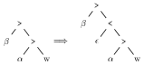
Figure 1: Decomposition in pictures
- Exercises
- Decompose the following lexical items at the vertical bar
- \(\epsilon\mathrel{::}\bullet V.k\bullet\mid{}d\bullet.v\)
- \(\textsf{give}\mathrel{::}\bullet d.k\bullet\mid{}d\bullet.V\)
Decomposition and Generalization
The entire point about this sort of lexical decomposition can be summarized in the following way:
lexical decomposition allows us to express regularities in the lexicon as new lexical items
If we measure the size of a grammatical description in terms of the number of features used (i.e. the sum of all features on all lexical items), then lexical decomposition can be used to reduce the size of our lexicon, by reifying repeated feature sequences as separate lexical items. Consider the set of lexical items in figure 1.
| \(\texttt{will}\mathrel{::}\bullet v.k\bullet.s\) | \(\texttt{must}\mathrel{::}\bullet v.k\bullet.s\) |
| \(\texttt{had}\mathrel{::}\bullet perf.k\bullet.s\) | \(\texttt{was}\mathrel{::}\bullet prog.k\bullet.s\) |
| \(\texttt{has}\mathrel{::}\bullet perf.k\bullet.s\) | \(\texttt{is}\mathrel{::}\bullet prog.k\bullet.s\) |
Each of these six lexical items has three features, giving us a total lexical size of 18. However, all six lexical items end with the same length two sequence of features: k•.s. This expresses that they check the case of a subject, and are a sentence; in even more naïve terms each lexical item demands that the subject moves to its specifier. We can decompose our lexical items so as to factor this common feature sequence out, giving rise to the lexicon in figure 2.
| \(\textsf{will}\mathrel{::}\bullet v.t\) | \(\textsf{must}\mathrel{::}\bullet v.t\) |
| \(\textsf{had}\mathrel{::}\bullet perf.t\) | \(\textsf{was}\mathrel{::}\bullet prog.t\) |
| \(\textsf{has}\mathrel{::}\bullet perf.t\) | \(\textsf{is}\mathrel{::}\bullet prog.t\) |
| \(\epsilon\mathrel{::}\bullet t.k\bullet.s\) |
This lexicon has seven lexical items, but only fifteen features. We can see that decomposition has reified the repeated feature sequence as a new lexical item, which expresses the generalization that subjects move to a specifier position at (or above) TP.
- Exercises
-
Identify and decompose redundancies in the following set of lexical items.
\(\textsf{John}\mathrel{::}d. k\) \(\textsf{Mary}\mathrel{::}d. k\) \(\textsf{the}\mathrel{::}\bullet n. d. k\) \(\textsf{every}\mathrel{::}\bullet n. d. k\) \(\textsf{no}\mathrel{::}\bullet n. d. k\) \(\textsf{some}\mathrel{::}\bullet n. d. k\) -
Give a preliminary analysis of the Saxon genitive construction in English (NP’s N):
- John’s doctor
- every man’s mother
Crucially, the NP to the left of the ’s cannot undergo movement.
-
Decomposition and Syntactic Word-Formation
Our decomposition scheme as described above treats the two parts of lexical items (their phonological and syntactic forms) asymmetrically; the syntactic feature sequence is split, but the phonological segment sequence is not. We can imagine, however, wanting to factor out redundancy, not only within feature bundles, but within the relation between phonological forms and feature bundles. Consider the pair of lexical items in figure 3.
| \(\textsf{is}\mathrel{::}\bullet prog.k\bullet.s\) | \(\textsf{been}\mathrel{::}\bullet prog.perf\) |
Not only do both of these lexical items begin with a • prog feature, but (we know) they are all forms of the auxiliary verb be. This generalization is, however, not expressed in the language of our theory (i.e. in terms of our lexicon). We would like to factor out the auxiliary from its endings. Abstractly, we need a decomposition rule like the following:
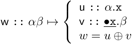
Figure 2: Morphemic decomposition
This rule would allow us to split a lexical item into two, but now the original phonological form of the lexical item (w) is factored into two pieces (u and v). The resulting pair of lexical items no longer give us the same structures we would have created with the original one, as now there are two heads (a u and a v) instead of just one (w), and in addition all specifiers in α intervene between these two heads. In order to remedy this problem, we must allow u and v to combine to form w. We do this in two steps. First, when merging expressions headed by u and v respectively, we combine the phonological material from both heads, and put them together into just one of the two.1 Second, we record that these two heads are not pronounced separately as u and v, but are rather pronounced together as w. This is done in two ways. First, in the lexical entry for v (the selector), we record (by underlining the relevant feature) that it enters into a special relationship with the head of its selected argument (• x). Second, we record that u and v are jointly pronounced as w.2 This latter is, in linguistic theory, the provenance of morphology. It is simply represented here as a finite list of statements (morphology can be thought of as a way of compressing this list, or alternatively a way of identifying and expressing rule-like generalizations). Using this decomposition rule, we obtain the lexical items in figure 4.
| \(\textsf{s}\mathrel{::}\underline{\bullet v}.k\bullet.s\) | \(\textsf{en}\mathrel{::}\underline{\bullet v}.perf\) |
| \(\textsf{be}\mathrel{::}\bullet prog.v\) | |
| \(is = be \oplus s\) | \(been = be \oplus en\) |
Complex heads
Once we move from whole word syntax to one which manipulates sub-word parts,3 we must confront two questions.
- how do the heads which constitute a single word get identified?
- where does the word corresponding to multiple distinct heads get pronounced?
The answer to the first question we gave implicitly in the previous section: two heads are part of the same word just in case one selects for the other with an underlined feature. There are many possible answers to the second question. Following Brody00, we say that a word is pronounced (relative to other words) as though it occupied the position of the highest of its heads (with respect to c-command) with a particular property (and in the lowest of its heads, if none have that property). This property is called strength in Brody’s work, but is formally merely an ad hoc property of lexical items. To distinguish between strong and weak lexical items, we write strong lexical items with two colons separating their phonological and syntactic features, and weak ones with one (as in figure 5).
| \(\textsf{u}\mathrel{::}\alpha\) | \(\textsf{v}\mathrel{:}\beta\) |
Decomposition and Learning
Decomposition can be thought of as a part of a learning mechanism for minimalist grammars. In particular, it provides a principled route from a whole-word syntactic analysis to the sort of decompositional syntactic analysis which is characteristic of minimalist-style analyses.
It is known that learning can take place in minimalist grammars in a highly supervised setting KobeleEtAl02,StablerEtAl03, where
- words are segmented into morphemes
- ordered and directed dependencies link words
which are in a feature checking relationship
- the \(i^{th}\) dependency of word u connects it to the \(j^{th}\) dependency of word v just in case the \(i^{th}\) feature of word u was checked by the \(j^{th}\) feature of word v
- the source of the dependency is the attractor feature, and the target of the dependency is the attractee feature
In this setting, the learner is given (essentially) full lexical items where feature names are unique to a particular dependency, and the learner’s task is to identify which feature distinctions should be kept, and which should be collapsed. In the cited works (following Kanazawa98), the pressure to collapse distinctions is provided by a limit on the number of homophones in the grammar.
We can use our decomposition mechanism to relax the supervision provided by the segmentation of words into morphemes (point 1). Accordingly, we assume that we are provided with sentences based on whole words, with dependency links between them as described by point 2 above.
Investigating English auxiliaries
As a simple case study, consider the English auxiliary system. Imagine the learner being exposed to sentences like the following.
- John eats.
- John will eat.
- John has eaten.
- John will have eaten.
- John is eating.
- John will be eating.
- John has been eating.
- John will have been eating.
The dependencies for sentence 8 are as in 3.
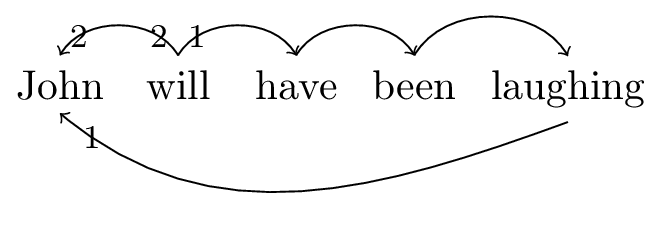
Figure 3: Dependencies for sentence ‘John will have been eating’
From these dependencies, we can reconstruct the lexical items in figure 6 Here, the names of the features are arbitrary.
| \(\textsf{John}\mathrel{::}a.b\) | \(\textsf{will}\mathrel{::}\bullet c. b\bullet.s\) |
| \(\textsf{have}\mathrel{::}\bullet d. c\) | \(\textsf{been}\mathrel{::}\bullet e. d\) |
| \(\textsf{laughing}\mathrel{::}\bullet a. e\) |
After extracting lexical items from sentences 1 –
8, we have multiple ‘copies’ of certain words, which differ
only in the names (but not the types) of features in their feature
bundles. For example, there are eight (!) different copies of John,
four of eating, three of will, and two each of eaten, has, and
been. We can unify these copies into single lexical items by
renaming the features involved across the whole lexicon. For example,
we might decide to rename the first feature of each of the John
lexical items to d, which would force us to replace all
features with name a with the name d, among others. After this
unification procedure, we are left with the lexicon on figure
7.
| \(\textsf{John}\mathrel{::}d. k\) | \(\textsf{eats}\mathrel{::}\bullet d. k\bullet.s\) |
| \(\textsf{will}\mathrel{::}\bullet v.k\bullet.s\) | \(\textsf{eat}\mathrel{::}\bullet d. v\) |
| \(\textsf{has}\mathrel{::}\bullet perf.k\bullet.s\) | \(\textsf{eaten}\mathrel{::}\bullet d. perf\) |
| \(\textsf{is}\mathrel{::}\bullet prog.k\bullet.s\) | \(\textsf{eating}\mathrel{::}\bullet d. prog\) |
| \(\textsf{have}\mathrel{::}\bullet perf. v\) | \(\textsf{be}\mathrel{::}\bullet prog.v\) |
| \(\textsf{been}\mathrel{::}\bullet prog. perf\) |
This grammar is perfectly capable of deriving the sentences (with the appropriate dependencies) we were given originally. However, it systematically misses generalizations: although we know (as English speakers) that there is a single verb, eat, which is appearing in its various forms in this lexicon, this fact is not captured in the grammar. Although this feels right, it is a somewhat wishy-washy argument. A more concrete (although less intuitively appealing) argument to the effect that there are missed generalizations, is that in order to add a new verb to our grammar we would need to add four separate lexical items (six, if we had included the past tense and the passive voice), one for each cell in its (derivational) paradigm.
We thus want to express generalizations about our language in terms of our theory, and this we will do via decomposition. There are many ways to begin; we want to compare pairwise lexical items to one another which have similar prefixes/suffixes and (ideally) similar phonologies. We should then decompose, and unify, decompose, and unify, until further decomposition does not achieve any succinctness gains.4 However we will here simply note en masse that the eat verbs begin with eat, and with the feature • d, and decompose them. The result is shown in figure 8
| \(\textsf{John}\mathrel{::}d. k\) | \(\textsf{s}\mathrel{::}\underline{\bullet v}.k\bullet.s\)\(\textsf{s}\mathrel{::}\underline{\bullet V}.k\bullet.s\) |
| \(\textsf{will}\mathrel{::}\bullet v.k\bullet.s\) | \(\epsilon\mathrel{::}\underline{\bullet V}.v\) |
| \(\textsf{has}\mathrel{::}\bullet perf.k\bullet.s\) | \(\textsf{en}\mathrel{::}\underline{\bullet V}.perf\) |
| \(\textsf{is}\mathrel{::}\bullet prog.k\bullet.s\) | \(\textsf{ing}\mathrel{::}\underline{\bullet V}.prog\) |
| \(\textsf{have}\mathrel{::}\bullet perf. v\) | \(\textsf{be}\mathrel{::}\bullet prog.v\) |
| \(\textsf{been}\mathrel{::}\bullet prog. perf\) | \(\textsf{eat}\mathrel{::}\bullet d. V\) |
| \(eats = eat \oplus s\) | \(eaten = eat \oplus en\) |
| \(eating = eat \oplus ing\) | \(eat = eat \oplus \epsilon\) |
Note that the original bare eat form has also been decomposed, leaving behind a ‘dummy’ lexical item which serves to simply change category. This is important, so that no new forms are derived: decomposition does not change the language of the grammar.
In the next step, we do the same with the forms of be.5 This is shown in figure 9.
| \(\textsf{John}\mathrel{::}d. k\) | \(\textsf{s}\mathrel{::}\underline{\bullet v}.k\bullet.s\)\(\textsf{s}\mathrel{::}\underline{\bullet V}.k\bullet.s\) |
| \(\textsf{will}\mathrel{::}\bullet v.k\bullet.s\) | \(\epsilon\mathrel{::}\underline{\bullet V}.v\) |
| \(\textsf{has}\mathrel{::}\bullet perf.k\bullet.s\) | \(\textsf{en}\mathrel{::}\underline{\bullet V}.perf\) |
| \(\textsf{s}\mathrel{::}\underline{\bullet x}.k\bullet.s\) | \(\textsf{ing}\mathrel{::}\underline{\bullet V}.prog\) |
| \(\textsf{have}\mathrel{::}\bullet perf. v\) | \(\epsilon\mathrel{::}\underline{\bullet x}.v\) |
| \(\textsf{en}\mathrel{::}\underline{\bullet x}.perf\) | \(\textsf{eat}\mathrel{::}\bullet d. V\) |
| \(\textsf{be}\mathrel{::}\bullet prog. x\) | |
| \(eats = eat \oplus s\) | \(eaten = eat \oplus en\) |
| \(eating = eat \oplus ing\) | \(eat = eat \oplus \epsilon\) |
| \(been = be \oplus en\) | \(be = be \oplus \epsilon\) |
| \(is = be \oplus s\) |
There are three as yet unjustified moves just made:
- the two ε forms are unifiable, but have not been
- the two en forms are unifiable, but have not been
- the two s forms are unifiable, but have not been
Regarding the first, the ε forms serve solely to assert isa
relationships between categories (every expression of type V is a
expression of type v). These must not be unified, as their presence
preserves the syntactic distinctions present in the input
sentences.6
There are three basic possibilities for dealing with the two en
forms:
- unify
Vandx - assert that
Visax - assert that
xisaV
Pursuing options 1 or 3 would collapse necessary syntactic
distinctions, leading the grammar to generate sentences of the form:
John will be (being)* eating. The correct option is 2. This can
be determined in a less intuitive manner by identifying cycles in
selection (or the lack thereof) in the lexicon: a V can be turned
into a prog (via ing), which can be turned into an x (via be),
but an x cannot become a V.7 The same reasoning applies to the
two s forms. Adding this information (as an empty lexical item) to
our lexicon gives us the lexicon in figure
10.
| \(\textsf{John}\mathrel{::}d. k\) | |
| \(\textsf{will}\mathrel{::}\bullet v.k\bullet.s\) | \(\epsilon\mathrel{::}\underline{\bullet V}.x\) |
| \(\textsf{has}\mathrel{::}\bullet perf.k\bullet.s\) | |
| \(\textsf{s}\mathrel{::}\underline{\bullet x}.k\bullet.s\) | \(\textsf{ing}\mathrel{::}\underline{\bullet v}.prog\) |
| \(\textsf{have}\mathrel{::}\bullet perf. v\) | \(\epsilon\mathrel{::}\underline{\bullet x}.v\) |
| \(\textsf{en}\mathrel{::}\underline{\bullet x}.perf\) | \(\textsf{eat}\mathrel{::}\bullet d. V\) |
| \(\textsf{be}\mathrel{::}\bullet prog. x\) | |
| \(eats = eat \oplus s\) | \(eaten = eat \oplus en\) |
| \(eating = eat \oplus ing\) | \(eat = eat \oplus \epsilon\) |
| \(been = be \oplus en\) | \(be = be \oplus \epsilon\) |
| \(is = be \oplus s\) |
We turn now to have, which results in the lexicon in figure 11.
| \(\textsf{John}\mathrel{::}d. k\) | |
| \(\textsf{will}\mathrel{::}\bullet v.k\bullet.s\) | \(\epsilon\mathrel{::}\underline{\bullet V}.x\) |
| \(\textsf{s}\mathrel{::}\underline{\bullet y}.k\bullet.s\) | |
| \(\textsf{s}\mathrel{::}\underline{\bullet x}.k\bullet.s\) | \(\textsf{ing}\mathrel{::}\underline{\bullet v}.prog\) |
| \(\epsilon\mathrel{::}\underline{\bullet y}.v\) | \(\epsilon\mathrel{::}\underline{\bullet x}.v\) |
| \(\textsf{en}\mathrel{::}\underline{\bullet x}.perf\) | \(\textsf{eat}\mathrel{::}\bullet d. V\) |
| \(\textsf{have}\mathrel{::}\bullet perf. y\) | \(\textsf{be}\mathrel{::}\bullet prog. x\) |
| \(eats = eat \oplus s\) | \(eaten = eat \oplus en\) |
| \(eating = eat \oplus ing\) | \(eat = eat \oplus \epsilon\) |
| \(been = be \oplus en\) | \(be = be \oplus \epsilon\) |
| \(is = be \oplus s\) | \(has = have \oplus s\) |
| \(have = have \oplus \epsilon\) |
Again, decomposition has given rise to two unifiable instances of the
morpheme s. There are the same three options, and searching for the
patterns of connectivity in the lexicon between y and x
demonstrate that x can become a y (via the route
be–en–have) but y cannot become an x. Thus we assume that
x isa y, as is shown in figure 12.
| \(\textsf{John}\mathrel{::}d. k\) | |
| \(\textsf{will}\mathrel{::}\bullet v.k\bullet.s\) | \(\epsilon\mathrel{::}\underline{\bullet V}.x\) |
| \(\textsf{s}\mathrel{::}\underline{\bullet y}.k\bullet.s\) | |
| \(\epsilon\mathrel{::}\underline{\bullet x}.y\) | \(\textsf{ing}\mathrel{::}\underline{\bullet v}.prog\) |
| \(\epsilon\mathrel{::}\underline{\bullet y}.v\) | |
| \(\textsf{en}\mathrel{::}\underline{\bullet x}.perf\) | \(\textsf{eat}\mathrel{::}\bullet d. V\) |
| \(\textsf{have}\mathrel{::}\bullet perf. y\) | \(\textsf{be}\mathrel{::}\bullet prog. x\) |
| \(eats = eat \oplus s\) | \(eaten = eat \oplus en\) |
| \(eating = eat \oplus ing\) | \(eat = eat \oplus \epsilon\) |
| \(been = be \oplus en\) | \(be = be \oplus \epsilon\) |
| \(is = be \oplus s\) | \(has = have \oplus s\) |
| \(have = have \oplus \epsilon\) |
This lexicon has 24 features in it (18, if we discount the isa lexical items), whereas the initial lexicon (prior to decomposition) contained 26 features. We have thus achieved a (small) compression. However, the important difference between these two lexica lies in their behaviour as more words are added to them; open class words such as intransitive verbs contribute just two features to our final lexicon, but 9 features (distributed over four lexical items) to our initial one.
Bibliography
[Brody00] “Michael Brody”, Mirror Theory: Syntactic Representation in Perfect Syntax, LI, 31(1), 29-56 (2000). ↩
[KobeleEtAl02] Gregory Kobele, Travis Collier, Charles Taylor & Edward Stabler, Learning Mirror Theory, in in: Proceedings of the Sixth International Workshop on Tree Adjoining Grammars and Related Frameworks (TAG+6), \emphVenezia, edited by (2002) ↩
[StablerEtAl03] @InCollectionStablerEtAl03, author = Edward P.~Stabler and Travis C.~Collier and Gregory M.~Kobele and Yoosook Lee and Ying Lin and Jason Riggle and Yuan Yao and Charles E.~Taylor, title = The Learning and Emergence of Mildly Context Sensitive Languages, booktitle = Advances in Artificial Life, pages = 525-534, publisher = Springer, year = 2003, editor = Wolfgang Banzhaf and Thomas Christaller and Peter Dittrich and Jan T.~Kim and Jens Ziegler, volume = 2801, series = Lecture Notes in Computer Science ↩
[Kanazawa98] “Makoto Kanazawa”, Learnable Classes of Categorial Grammars, CSLI Publications (1998). ↩
-
Just which head should host the phonological material is something we shall address in a bit. ↩︎
-
It would make sense as well to, upon combining u and v, to replace them with w. I prefer, when doing theory construction, to factor out logically distinct steps: syntax will then assemble complex heads, and these complex heads will be interpreted elsewhere. Of course, when actually using this theory to model performance, these logically distinct steps can and perhaps should be interleaved with one another. ↩︎
-
In current parlance, this would be described as moving from a pre-syntactic morphological module to a post-syntactic one. ↩︎
-
This is easier said than done! Marina Ermolaeva is working on this. ↩︎
-
There is a deep issue here, regarding how we are to know that is is a form of be. There has been computational work on identifying morphological paradigms JLee14, which might very well be of use here. ↩︎
-
They can be replaced by partial ordering statements of the form \(V \le v\) and \(x \le v\) (see SzabolcsiBernardi08). ↩︎
-
This is unfortunately quite a bit more complicated. An
xcould in principle become aV, if it were embedded as a clausal complement, or as a relative clause modifier of a DP complement, of a higher verb. ↩︎